Simulating The Ronchi Test
Understanding The Inner Workings Of Ronchi For Windows
John D. UptonMay 15, 2000
Here, you can learn about the internal workings of a simulation program for the Ronchi Test. These are the techniques that have gone into the Freeware program Ronchi for Windows. You can duplicate these formulae and techniques in your own Ronchi program while adding the features you need or desire. You may also find this information valuable in other ATM programming pursuits as well.
An Overview Of The Ronchi Test
The Ronchi test is much like the Foucault test in its set-up. Unlike the Foucault test, however, the Ronchi test is not inherently quantitative. It cannot tell you exactly how good (or bad) you mirror actually is. It does easily show all the mirror's zones and irregularities. It can also give you a very good feeling for the overall quality of your mirror and can give you all that information at a glance. That is where the test really shines. You may use the test to get that clear, quick overview of the shape of your mirror as a whole. You would then normally want to run some other quantitative test against your mirror to determine whether you have met your desired quality criteria.
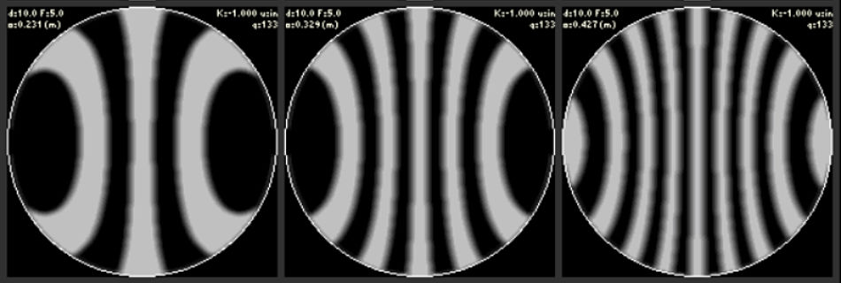
To run the Ronchi test, you need a small pinhole or slit light source which illuminates the mirror under test and a knife edge carriage in the path of the returning light from the mirror. Both the light source and the carriage are placed near the radius of curvature of the mirror. In the Ronchi test, the actual knife edge is replaced by a fine grating consisting of opaque lines ruled onto a transparent substrate. The mirror's surface is viewed through this grating. As the carriage is moved slightly toward and away from the mirror, the lines on the grating which appear projected onto the surface of the mirror will change in response to the new configuration. For a spherical mirror, the lines will appear straight and undistorted. For any shape other than spherical, the lines will appear bent in an amount and direction dependent on the mirror diameter, its radius of curvature, its conic shape, the grating's line density, and the placement of the grating with respect to the radius of curvature point. Figure 2 below shows some typical Ronchi test images at several different grating offsets.
In recent years, there has been a movement towards making the Ronchi test more quantitative. The newer method of running the test has been termed the Matching Ronchi test. While it is still fundamentally qualitative, the Matching Ronchi test attempts to be able to apply some criteria to the testing so that the result is a bounding of the quality of the mirror. The new method of using the test does this by having the operator match the appearance of their mirror to a perfect mirror having exactly the same specifications as their own. When the two match, you are done. Finding or making such a comparison mirror would seem an impossible task. That is where the modern Personal Computer enters the scene. A computer is capable of creating just such a perfect mirror and showing the test operator what their mirror should look like.
The Matching Ronchi test is easy to perform. You create a virtual, perfectly figured mirror with the same specifications as your own on the computer screen and then visually verify that your in-process mirror looks the same. Since the distortion of the bands depends on several factors, to ensure an actual match, you must compare your mirror and the virtual mirror at three or more different offsets. When the two match at all offsets you compare, then your mirror is done. Further, you can get some idea of how accurate your mirror is if you can also compare it to several virtual mirrors with a known amount of error. In this way, it is possible to assign an upper quantitative bound to the accuracy of your mirror using a qualitative test. This is the basis for the Matching Ronchi test.
The only task that remains is to write a computer program that can simulate the appearance of a perfect mirror undergoing the Ronchi test. Taking this one step further, the program can also calculate the appearance of a mirror with a known amount of error. Two such virtual mirrors can then be used to set the bounds the user works within to achieve their desired quality criteria. These are the key tasks performed inside the Freeware program Ronchi for Windows.
The Geometry Of The Simulation
The fundamental task of simulating the distortion of the grating's lines in the Ronchi test can be approached from simple geometry. In the discussion that follows, I will freely (and sloppily) use the absolute value of many of the quantities in order to keep the steps clear and concise. If you wish to write a program based on this information, you must pay close attention to sign conventions. (The computer is much less forgiving than the human mind in this respect.) Figure 3 below shows two views of the Ronchi test. The view at the left represents the view the user has while performing the Ronchi test. The view is from the perspective of the tester looking at the face of the mirror. The right view is a plan view from the top looking down on the test set-up.
Imagine a ray of light leaving the tester's source at the radius of curvature and hitting the mirror. If the mirror is spherical, that ray will return to the light source. In practice, the light source may be moved slightly away from the optical axis so that the returning ray may be viewed. Most ATMs may prefer to move the source down a small amount and view the returning light over the top of the source. This makes it easily visible and avoids some of the effects of moving the source to one side. For the purposes of simulation, however, it will be assumed that everything is precisely on axis. In addition, the simulation will assume that the light source and grating move as a unit. This is the so called moving source tester design. A fixed source (but moving grating) tester may be approximated by halving the grating offsets input for the simulation.
In the left view in Figure 3, assume that a light ray hits the mirror at point P. Assuming the origin is at the center of the mirror, that ray has an x offset of Px, a y offset of Py, and hits the mirror at a zonal radius of Pr. By definition, the radius of curvature of the central zone of the mirror is R. Any ray that hits the mirror at a zonal radius Pr from the center of the mirror will cross the optical axis at a point b * s away from R, where b is the coefficient of deformation and s is the sagitta of the mirror at that zonal radius. (The quantity b is also known as the Schwarzchild Constant, SC, or the Conic Constant, K, for the curve.)
Next, we need to consider the grating which is placed a short distance from the radius of curvature of the mirror. We will call this distance o for offset. To complete the definition of quantities, let g represent the line width of the grating. This is the width of a single opaque line in the grating. We will define the edge length as the width of the individual lines and gaps of the grating.
g = 1.0 / (2.0 * lines) eq. 1
The lines parameter is the specified number of lines per unit length on the grating -- such as 100 lines per inch.
Figure 4 shows a magnified view of the area near the radius of curvature. This view is again from the top looking down on the test set-up. Using Figure 4, we can now derive the formulae which define the method to "ray trace" the grating's shape as projected onto the mirror.
First, note that for a light ray striking any point P on the mirror's surface, the reflected ray will cross the axis at point R + (b * s). Note also that the grating is placed at a distance o from R. We must remember, though, that we are only interested in how far the returning ray is from the optical axis in the x direction. This is because the lines of the grating are at fixed distances from the yz plane which includes the optical axis. As can be seen in the two prior diagrams, the ray is coming from a point that is a distance Px from the optical axis in the x direction.
To begin the simulation, let's first calculate the quantity b * s since it is used several places in the calculations. For a paraboloid, the sagitta is given by
s = (Pr * Pr) / (2.0 * R) eq. 2
For any arbitrary conic, the more general formula for the sagitta is
s = (Pr * Pr) / (R * (1.0 + Sqrt(1.0 - ((Pr * Pr) / (R * R)) * (b + 1.0)))) eq. 3
Now, we should be able to find the point at which the ray intersects the grating. Let's let Lx represent the lateral offset in the x direction of the ray at the point it passes through the grating. From similar triangles, we can see that
Px / (R + (b * s)) = Lx / ((R + o) - (R + (b * s))) eq. 4
Thus for any ray striking the mirror at point P, the ray will pass through the grating at a point
Lx = Px * (o - (b * s)) / (R + (b * s)) eq. 5
Now that we know where the ray laterally intersects the grating, we need to see if it will intersect an opaque line or a transparent area. In the first case, the point P on the mirror will appear dark, while in the second case, it will appear bright. Figure 5 at left helps us determine where the ray has crossed. It represents a highly magnified view of the grating aligned on the optical axis. Recall above that the quantity g was defined to be the width of a single opaque or transparent area on the grating. Note in the diagram that the grating is centered on the optical axis. Because of this, we must account for the g / 2.0 offset to the first edge of a grating line when we make our calculations.
At this point we will define a new quantity V to represent the visibility of the light ray coming from point P on the mirror. Once we move the origin from the optical axis to the first edge at g / 2.0, we can see that Lx / g will tell us where the ray transverses the grating. Thus we can write the expression V = (Lx - (g / 2.0)) / g which will tell us about the ray's visibility. This is made easier if we only look at the integer result of this operation and ignore the remainder. Using the integer result of this division, we see that if the result is 0 or even, then the ray will be visible. If the result is odd, then the ray will be blocked from our view by the line on the grating. We can also optionally invert (even / odd) this visibility result to simulate the grating being aligned with a transparent area on the optical axis.
Performing The Ronchi Test Simulation
The procedure for drawing the image can finally be summarized as follows:
- Pick a point P on the mirror's surface. You may want to just pick random points as in many ray trace tools, or you can calculate every point. Ronchi for Windows calculates every point on the mirror at whatever screen resolution the user has chosen.
- Calculate the zonal radius Pr for your point using the Pythagorean theorem.
- Pr = Sqrt((Px * Px) + (Py * Py)).
- Make sure that the point you picked is really on the mirror.
- Pr <= mirror_radius
- Calculate the point at which this ray crosses the optical axis beyond the radius of curvature.
- b * s = (b * Pr * Pr) / (2.0 * R)
- Recall that this is only valid for a paraboloid. If your target mirror is not close to a paraboloid, you should use the other more general formula given earlier.
- Calculate the lateral distance from the optical axis where the ray intersects the grating.
- Lx = Px * ((b * s) - o) / (R + (b * s))
- Determine whether the ray intersects an opaque or transparent area of the grating.
- V = (Lx - (g / 2.0)) / g
- Draw the point on the mirror's image in the proper color.
- Process as many other points on the mirror's surface as required using these same steps.
Making The Ideal Image More Realistic
The above method calculates the ideal appearance of the Ronchi grating's shadow bands across the face of the mirror. We have assumed a point source and ignored the effects of diffraction. Both of these factors affect the true appearance of a mirror under the Ronchi test. If it is desirable to have a somewhat more realistic appearance to the simulation, further processing of the Ronchi images may be done. (Of course one could also use wave optics theory rather than geometry to generate the image. In that case, no further processing would be required.)
There are (at least) three similar methods for processing the image to give a more realistic appearance. Each is just a way of defocussing the image and optionally applying some artistic license to model diffraction effects. The first method is to assume a finite width slit and calculate each mirror point as many times as required to model the width of the slit. Each of these intermediate calculations is added together to get the resultant intensity color of the image at that point. The second method also assumes a finite width slit and then assumes that the mirror's image from each sliver of the slit is just added together. In this method the image is calculated once per the above standard method and then added to an offset version of itself a number of times simulating the addition of multiple slit image increments.
Each of these methods has drawbacks in coding, so Ronchi for Windows uses an approach used in more traditional image processing applications. This is the third method. It consists of processing each pixel in the ideal Ronchi image using a modified blur filter. The blur filter is modified from its usual form to help account for diffraction effects in the image. While not an accurate representation of diffraction, it results in an image which at least reminds the user somewhat of how diffraction effects appear in the Ronchi test.
The size of the blur filter is changed as screen resolution changes, but its general form remains the same. It can be represented by the matrix shown at upper left. This differs from the traditional blur filter primarily in that it is not symmetrical. The filter is a bit wider in the x direction than it is in the y direction. This tends to blur the image more across its diameter than in its height. While it is not very asymmetrical, its effects are visible on the screen and it gives a more pleasing appearance to the resulting image.
The absolute size of the matrix is determined by the current screen image size. By keeping the matrix size a certain percentage of screen resolution, the image blurring appears natural regardless of size. (You probably would not want to apply a 10 by 10 blur filter to an image only 50 pixels wide.) In use, the filter is applied to each point in the ideal image by using the matrix to multiply each pixel by its neighbors, sum, and then normalize the point. Attention must be paid to boundary conditions during the application of the blur filter. After applying the filter to every point in the ideal image, the result is then displayed as the "realistic" Ronchi image for the user.
Calculating The Error Criteria
The final step in our simulation is to determine the parameters required to simulate a less than perfect mirror. Here it is easiest to assume that the mirror under test is at least a smooth conic curve of some sort. Zonal aberrations such as turned edge or higher order aberrated zones cannot be easily simulated using the methods outlined above. For that reason, we will take the easy way out and assume the user is approaching a paraboloid with a smooth under or over corrected conic shape.
Once the user specifies their error criteria, we can calculate the equivalent Conic Constant b which describes a curve which deviates from the mirror's desired shape by precisely the amount specified. It is then simply a matter of simulating the new mirror to show the user what to look for. It is actually better to show the user two such mirrors, one over corrected by their criteria and one under corrected by the same amount. This visually bounds the degree of matching the user must achieve.
In order to make this error calculation, we go back to the general form of the equation for the sagitta of any conic presented earlier.
s = (Pr * Pr) / (R * (1.0 + Sqrt(1.0 - ((Pr * Pr) / (R * R)) * (b + 1.0))))eq. 3
This time we will be dealing with the full mirror, so we will use r, the mirror's radius, in place of Pr, the point's zonal radius. Let's also define the quantity W, for surface wave error. Note that the surface wave error is actually a length measurement and must be translated to such from the users wave criteria. Also note that usual convention dictates that the wavefront error is what the user should specify and that quantity needs to be halved to give the surface error criteria allowed. The surface with applied error we are looking for can be described as
s2 = s1 ± W eq. 6
where s2 is the aberrated surface and s1 is the perfect surface we seek for our mirror. Expanding s2 using the general conic equation gives us
(r * r) / (R * (1.0 + Sqrt(1.0 - ((r * r) / (R * R)) * (b + 1.0)))) = s1 ± W eq. 7
Now we can solve for the b which corresponds to that aberrated mirror. Rearranging terms, we get
b = ((R * R) / (r * r)) * ((2.0 * z) - (z * z)) - 1.0 eq. 8
where the intermediate quantity z is defined by
z = (r * r) / (R * (s1 ± W)) eq. 8a
All that remains now is to generate and display the Ronchi images using the two b values that are calculated. (You may optionally allow calculations with an error of four times the user specified amount in order to allow for refocussing of the image at the telescope. This corresponds to choosing a slightly different reference curve and focal length for the mirror.)
There you have it. Overall, the math involved in writing a Ronchi test simulator is not overly complex. As in any computer programming task, the real work is making the program easy to use, crash proof (as can be,) and fast. Those are the real challenges behind writing a program such as Ronchi for Windows. To download your copy of my Ronchi test simulator, get it from this site's download area. Ronchi for Windows software (zip file). Feel free to incorporate any of these techniques into your own program.